|
A random field is simply another name for a random function  , where , where  ranges over some
state space. As described in this
other coupling demonstration,
we can build Markov chains ranges over some
state space. As described in this
other coupling demonstration,
we can build Markov chains  by simply chaining together a series of independent random functions:
 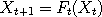 for for
 = 0, 1,2, 3 etc.
Each such function = 0, 1,2, 3 etc.
Each such function  has the same fixed probabilities of taking a particular value, i.e. there
exists a transition kernel has the same fixed probabilities of taking a particular value, i.e. there
exists a transition kernel  such that such that

Suppose now that we modify the functions in such a way as to keep these probabilities intact,
then by chaining those new functions which we now call  say, we obtain a Markov chain say, we obtain a Markov chain  which is statistically the same as but may have other new properties.
Whenever we want to make several chains, all of which have the same transition kernel ,
meet over time it makes sense to modify the original , replacing them with suitably chosen
which are designed to facilitate coalescence. Perfect simulation
requires such constructions, for
example. See also here. which is statistically the same as but may have other new properties.
Whenever we want to make several chains, all of which have the same transition kernel ,
meet over time it makes sense to modify the original , replacing them with suitably chosen
which are designed to facilitate coalescence. Perfect simulation
requires such constructions, for
example. See also here.
Suppose that we draw a graph of the functions  and and  . Since these functions are random,
the graphs will not always look the same, but certain qualitative features may still stand out. For example,
the graphs may be flat or horizontal in some places. In that case the locations which belong
to that region would all map to the same value, that is . Since these functions are random,
the graphs will not always look the same, but certain qualitative features may still stand out. For example,
the graphs may be flat or horizontal in some places. In that case the locations which belong
to that region would all map to the same value, that is  for all and for all and  within the region where the graph of is flat. If was used to drive two Markov chains
 and and  say, and if both say, and if both  and and  both happen to be inside this region, then we would have
  afterwards and forever. The Markov
chains have coupled. Obviously, the chance of coupling two random chains (which both use the same series )
increases the more flat areas exist in each . afterwards and forever. The Markov
chains have coupled. Obviously, the chance of coupling two random chains (which both use the same series )
increases the more flat areas exist in each .
If you press the button above, a separate window should open demonstrating this scheme in the context of
Markov chain Monte Carlo simulation. Starting with a random function
which is not necessarily flat anywhere, but has a given set of transition probabilities,
we generate successive modifications of this function by flattening randomly
chosen regions in such a way that we do not destroy these probabilities. The exact details are described in an
accompanying paper (ps/pdf). Eventually, we end up
with a `fully flattened' function to replace .
The controls of this applet are similar to those for the Metropolis-Hastings applet. The main window
under the target distribution contains the successive modifications of the random field whose transition
probabilities correspond to  , the proposal distribution for a Metropolis-Hastings algorithm.
The third and fourth panels on the left represent histograms of respectively the modified and unmodified random functions (also
called fields here) after metropolization. If you wait long enough, both histograms will look alike, as they should since the
transition probabilities have been preserved. , the proposal distribution for a Metropolis-Hastings algorithm.
The third and fourth panels on the left represent histograms of respectively the modified and unmodified random functions (also
called fields here) after metropolization. If you wait long enough, both histograms will look alike, as they should since the
transition probabilities have been preserved.
|